The modified homotopy perturbation method and its application to the dynamics of price evolution in Caputo-fractional order Black Scholes model

Abstract

Background

Following a financial loss in trades due to lack of risk management in previous models from market practitioners, Fisher Black and Myron Scholes visited the academic setting and were able to mathematically develop an option pricing equation named the Black–Scholes model. In this study, we address the solution of a Caputo fractional-order Black–Scholes model using an analytic method named the modified initial guess homotopy perturbation method.

Methodology

Foremost, the classical Black Scholes model relaxed for European option style is generalized to be of Caputo derivative. The introduced method is established by coupling a power series function of arbitrary order with the renown He’s homotopy perturbation method. The convergence of the method is demonstrated using the fixed point theorem, and its methodology is illustrated by solving a generalized theoretical form of the fractional order Black Scholes model. The applicability of the method is proven by solving three different fractional order Black–Scholes equations derived from different market scenarios and its effectiveness is confirmed as feasible series of arbitrary orders that accelerate fast to the exact solution at an integer order were obtained. The computation of these results was carried out using Mathematica 12 software. Subsequently, the obtained outcomes were utilized in Maple 18 software to conduct a series of numerical simulations. These simulations aimed to analyze the influence of the fractional order on the dynamics of payoff functions regarding the share value as the option approached its expiration date under varying market constraints. In all three scenarios, the results showed that option values decrease as the expiration date approaches the integer order. Furthermore, the comparative outcomes reveal that Caputo fractional order derivatives control the flexibility of the classical Black–Scholes model because its payoff curve exhibits more sensitivity to changes associated with market characteristic parameters, such as volatility and interest rates.

Recommendations

We propose that the results of this work should be examined and implemented by mathematicians and economists to better comprehend the influence of Caputo-fractional order derivatives in understanding the dynamics of option price evolution of financial assets.

1 Background

Options constitute one of the most frequently traded financial assets. The Black–Scholes model is an option pricing model that was proposed by Black and Scholes in [1, 2] and Merton in [3, 4]. This model showed the significance of mathematics in finance. It is a second-order parabolic partial differential equation that is often used to compute the theoretical values of financial options based on market features such as stock price, risk rate, strike price, and volatility rate.

Many researchers have contributed to the understanding and implementation of the Black–Scholes model in mathematical finance. For example, the authors of [5] investigated the numerical solution of the Black–Scholes model. They explored the comprehensive history of Black–Scholes model's, discussed the parameters of the model and their functions, and provided a numerical approach capable of determining the model's outcome. Their findings, which showed convergence with the precise value, were presented and discussed. A numerical method for pricing double-barrier options in a time-fractional Black–Scholes model was provided in [6] and an approach suitable for computing the exact solution of Black Scholes model was studied in [7]. The stability and convergence of the proposed numerical scheme were shown using Fourier analysis, and the results verified the method's usefulness in solving the Black–Scholes model. The dynamics of option pricing were explored in [4] using a modified Black–Scholes-Merton model for option pricing. In their work, they constructed a conformable model that allows additional flexibility for markets, and an empirical application is carried out.

Fractional calculus has recently piqued the interest of contemporary academics, especially in the modeling of phenomena like diseases and financial theories. This is primarily because it introduces greater flexibility, imparts a long-term memory effect, and lends a more realistic dimension to these phenomena [8,9,10,11]. Among the several fractional operators in use, notable ones include the Riemann–Liouville [12, 13], Caputo [14, 15], Caputo–Fabrizo [16], and Atangana–Baleanu [17] operators. These operators serve as versatile tools for exploring fractal and chaotic phenomena characterized by non-local kernels [18]. An in-depth discussion of these properties, advantages, and disadvantages of these operators can be found in [19], which provides several significant results of studies concerning a fractional optimal control problem in systems with time-delay arguments. Similarly, the results provided in [20] on fractional optimal control for variable-order differential systems give supportive insights on the efficacy of mathematical modeling using these derivatives. The impact of Caputo-fractional operators on financial asset option pricing is of special interest in this study. The original Black–Scholes model, which was established using the classical derivative, may be insufficient for examining the behavior of financial asset option prices over time. It is imperative that, for better prediction of future asset price movements, attention be paid to the repeated patterns and trends observed in financial data. In [21], there is empirical evidence backing the repeated patterns and trends in financial markets as associated with fractional order derivatives. As a result, to generalize the derivative of the traditional Black–Scholes model, researchers usually employ a non-localized derivative, such as the Caputo fractional operator proposed by [13] and implemented in [22].

Mathematicians frequently research alternate techniques for obtaining the fractional-order Black–Scholes model's solutions because it is often challenging to obtain the exact solution of the model analytically. Numerous researchers have utilized a variety of numerical approaches and strategies to obtain an approximate solution to the fractional-order Black–Scholes model. The homotopy perturbation method proposed in [23] is a prime example of this approach. This method has been widely employed by different researchers ever since its emergence. For example, [24] modified and applied the homotopy perturbation method to obtain the approximate solution of fractional order Korteweg-De Vries equation. The method proved effective and their results showed rapid convergence to the exact solution. In [4], this same homotopy perturbation method was applied on a fractional order Black–Scholes model described in Caputo sense. It yields an analytic solution in the form of a convergent series with readily computed components. Also, a numerical computation of fractional Black Scholes equation arising in financial market was presented in [25]. In their research, they applied the homotopy perturbation method and homotopy analysis method to solve fractional order Black Scholes Model and both methods proved to be highly effective as they both produce convergent series results. This homotopy perturbation approach was also applied in [26] to achieve an approximate analytical solution to a fractional-order Integro-differential equation. Their research indicated that the homotopy perturbation approach is a convergent and easily computable method for solving linear and non-linear fractional order models originating from application areas. A conformable fractional modified homotopy perturbation approach was employed in the study [27] to solve a novel European call option model. Their results showed that the proposed method is an efficient and powerful technique for finding approximate solutions to the fractional Black–Scholes models, which are considered conformable.

Although several studies on techniques for solving the fractional order Black–Scholes model have been published, the majority of the methods are not stable and are limited to different constraints. This motivates the necessity of providing an unconditionally stable and reliable method of solving the fractional-order Black–Scholes model in this study. Hence, we proposed a modified initial guess homotopy perturbation method [24, 28,29,30], which is a simple and effective analytical method to solve and investigate the behavior of the components associated with modern option pricing theory while utilizing less computational effort.

Thus consider the following fractional-order Black–Scholes differential equation.

$$\frac{{\partial^{\alpha } f(S,t)}}{{\partial t^{\alpha } }} + rS\frac{\partial f(S,t)}{{\partial S}} + \frac{1}{2}\sigma^{2} S^{2} \frac{{\partial^{2} f(S,t)}}{{\partial S^{2} }} - rf(S,t) = 0$$

(1)

For an European option, the solution of (1) as explained in [31, 32] is defined to be $f(S,t) = \max \left\{ {f_{ * } ,0} \right\}$. This represents the worth (contingent claim) of the asset where $f_{ * } = \pm \varsigma (S - E)$ and $\varsigma = \pm 1$ respectively stands for the European call and put option prices. The stock price is denoted with S, $E = Ke^{ - r(T - t)}$ embed parameters K, r, T, t representing the strike price, the riskless rate, the maturity date and the strike time of the option respectively. Expression $(f_{ * } ,0)^{ + }$ signifies the maximum value between f_* and zero. And the standard deviation (volatility rate) denoted by σ is a normally distributed parameter.

An alternative form of the classical order Black–Scholes model presented in [33, 34] was derived using the following transformation:

$$\left. {\begin{array}{*{20}l} {S = Ee^{x} ,} \hfill \\ {f(s,t) = Ev(x,t)} \hfill \\ {2\tau = (T - t)\sigma^{2} } \hfill \\ \end{array} } \right\}$$

(2)

Such that

$$\frac{\partial f}{{\partial t}} = - E\frac{{\sigma^{2} }}{2}\frac{\partial v}{{\partial \tau }},\quad \frac{\partial f}{{\partial S}} = \frac{E}{S}\frac{\partial f}{{\partial x}},\quad \frac{{\partial^{2} f}}{{\partial S^{2} }} = - \frac{E}{{S^{2} }}\frac{\partial v}{{\partial x}} + \frac{E}{{S^{2} }}\frac{{\partial^{2} v}}{{\partial x^{2} }}$$

Which yields

$$\frac{\partial v(x,t)}{{\partial t}} - (m - 1)\frac{\partial v(x,t)}{{\partial x}} - \frac{{\partial^{2} v(x,t)}}{{\partial x^{2} }} + mv(x,t) = 0$$

(3)

Modifying (3) by generalizing the classical integer order operator using the Caputo fractional order operator we obtain:

$$\frac{{\partial^{\alpha } v}}{{\partial t^{\alpha } }} - (m - 1)\frac{\partial v}{{\partial x}} - \frac{{\partial^{2} v}}{{\partial x^{2} }} + mv = 0$$

(4)

where $m = \frac{2r}{{\sigma^{2} }}$ represents the equilibrium of the free interest rate and stock market volatility [35].

1.1 Basic definitions

We discuss some essential features of fractional calculus applied in this study here.

Definition 1

A real function ψ(x), for x > 0, exists in the space $\delta_{\nu } ,\nu \in R$ if a real number $k > \nu$ exists such that $\psi (x) = x^{k} \psi_{1} (x)$. Where $\psi_{1} (x) \in \delta (0,\infty )$, and ψ(x) is said to exists in space $\delta_{v}^{\alpha }$ if and only if $\psi^{(\alpha )} \in \delta_{\nu } ,\alpha \in N$.

Definition 2

The Riemann–Liouville fractional integration of order $\gamma \ge 0$ for a real positive function $\psi (x) \in \delta_{\nu } ,\nu \ge - 1\,\,\,x > 0$ is defined as:

$$I^{\gamma } \psi (x) = \frac{1}{\Gamma (\gamma )}\int\limits_{0}^{x} {(t - x)^{\gamma - 1} \psi (t){\text{d}}t} .$$

The Riemann–Liouville fractional integral operator I^γ for $\psi (x) \in \delta_{\nu \,} ,\nu \ge - 1\,\,\,\gamma ,\alpha \ge 0$ and $\beta \ge - 1$ satisfies the following properties:

• 1. $I^{\gamma } I^{\alpha } \psi (x) = I^{\gamma + \alpha } \psi (x),$

• 2. $I^{\gamma } I^{\alpha } \psi (x) = I^{\alpha } I^{\gamma } \psi (x),$

• 3. $I^{\gamma } t^{\beta } = \frac{\Gamma (\beta + 1)}{{\Gamma (\gamma + \beta + 1)}}t^{\gamma + \beta } .$

Definition 3

For a positively defined real function $\psi (x) \in \delta_{\nu }$, the Caputo fractional derivative can mathematically be expressed as;$D^{\gamma } \psi (x) = \frac{1}{\Gamma (\alpha - \gamma )}\int\limits_{0}^{x} {(x - t)^{\alpha - \gamma - 1} \psi^{(\alpha )} (t){\text{d}}t} ,\quad \alpha - 1 < \gamma \le \alpha ,\quad \alpha \in N.$

The Caputo fractional derivative is a sort of regularization in the time origin for the Riemann–Liouville fractional derivative.

Lemma

Let $T > 0:u \in \left( {\left[ {0,T} \right]} \right),p \in \left( {m - 1,m} \right),m \in N\quad {\text{and}}\quad v \in c^{{\prime }} \left( {\left[ {0,T} \right]} \right)$. Then for $t \in \left[ {0,T} \right]$ the following properties hold:

$$\begin{aligned} D_{ + }^{p} v\left( t \right) & = \frac{{\text{d}}}{{{\text{d}}t}}I_{ + }^{1 - p} v\left( t \right) \\ D_{ + }^{p} I_{ + }^{p} v\left( t \right) & = v\left( t \right) \\ I_{ + }^{p} D_{0}^{p} & = u\left( t \right) - \sum\limits_{k = 0}^{m - 1} {\frac{{t^{4} }}{k!}u^{\left( k \right)} \left( 0 \right)} \\ \mathop {\lim }\limits_{{t \to 0^{ + } }} D_{0}^{p} u\left( t \right) & = \mathop {\lim }\limits_{{t \to 0^{ + } }} I_{ + }^{p} u\left( t \right) = 0 \\ \end{aligned}$$

And

$$D^{\gamma } \psi (t) = \frac{1}{\Gamma (1 - \gamma )}\int\limits_{t}^{T} {(x - t)^{ - \gamma } \psi^{{\prime }} (s){\text{d}}s}$$

Is the so called right fractional Caputo derivative which represents the future state of the function ψ(t). For more details on definitions and properties we refer to [19, 20, 36].

Theorem 1

Suppose there exist a contracting nonlinear mapping $\gamma :\delta \to \zeta$ specify on two Banach spaces, δ, ζ for all $\mu ,\nu \in \delta$, then $\left\| {\gamma (\mu ) - \gamma (\nu )} \right\|_{\zeta } \le \tau \left\| {\mu - \nu } \right\|_{\delta }$, for $0 < \tau < 1$ such that the sequence $\mu_{k + 1} = \gamma^{n} (\mu_{0} ) = \gamma (\mu_{0} )$ for some $\mu_{0} \in \delta$ which converges to a unique fixed point γ [37].

Proof

Consider the Picard sequence $\mu_{k + 1} = \gamma (\mu_{k} ) \subseteq \zeta$ we want to show that μ_k is convergent in ζ for all $r \ge k$$\left\| {\mu_{k} - \mu_{r} } \right\| \le \left\| {\mu_{k} - \mu_{k + 1} } \right\| + \left\| {\mu_{k + 1} - \mu_{k + 2} } \right\| + \left\| {\mu_{k + 2} - \mu_{k + 3} } \right\| + \cdots + \left\| {\mu_{k - 1} - \mu_{r} } \right\|$.

The proof is defined by using mathematical induction on the contractive property of (C) such that $\left\| {\mu_{k} - \mu_{k + 1} } \right\| \le \tau^{k} \left\| {\mu_{0} - \mu_{1} } \right\|$. By implication, $\mathop {\lim }\limits_{r \to \infty } \left\| {\mu_{k} - \mu_{r} } \right\| \le \frac{{\tau^{k} }}{1 + \tau }\left\| {\mu_{0} - \mu_{1} } \right\| = 0\quad {\text{as}}\quad k \to \infty$.

This proves that (μ_k) is Convergent in ζ and through completeness of ζ, we can find $\Lambda \in \zeta$: $\mathop {\lim }\limits_{k \to \infty } (\mu_{k} ) = \Lambda \in \zeta$. Clearly, the continuity of γ is ensured by the contraction (C). Thus $\Lambda = \mathop {\lim }\limits_{k \to \infty } \mu_{k + 1} = \mu_{r}$.

2 Methods

2.1 Applied algorithm

In this section, we present the algorithm used to approximate solutions for the Black–Scholes model.

Algorithm

• 1. Define the Black–Scholes Model:

  • Define the input parameters: current stock price (S), strike price (K), time to expiration (T), risk-free interest rate (r), volatility (σ), and option type (call or put).

  • Determine whether dividends are involved in the model.

• 2. Create an Initial Guess Functional for the Option Price:

  • Construct an initial guess functional for the option price given by $u\left( {x,t} \right) = \lambda_{0} + \lambda_{1} t + \lambda_{1} t^{2} \cdots$

• 3. Repeat until convergence:

  • a. Evaluate the Black–Scholes Model using the Initial Guess Function to obtain the first approximation λ₁t

  • b. Construct a He's Homotopy Perturbation Correctional Functional which corrects the initial approximation to a more accurate estimate.

  • c. Evaluate the correctional functional with the first approximation to obtain the next approximation

  • d. Compute subsequent approximations using the previous approximations

  • e. Check for Convergence such that $\left| {u_{n + 1} \left( {x,t} \right) - u_{n} \left( {x,t} \right)} \right|$ is less that a predefined accuracy threshold ε

• 4. If the solution does not converge:

  • Output "Not Convergent."

  • Go to 3(d)

• 5. If the solution converges:

  • Output the approximate option price:

  • End.

  This algorithm presents a systematic process for estimating option prices by employing the Black–Scholes model and the modified He's homotopy perturbation method, and it concludes upon achieving a converged result. Figure 1 illustrates the algorithm's sequential flow, as depicted below.

  Fig. 1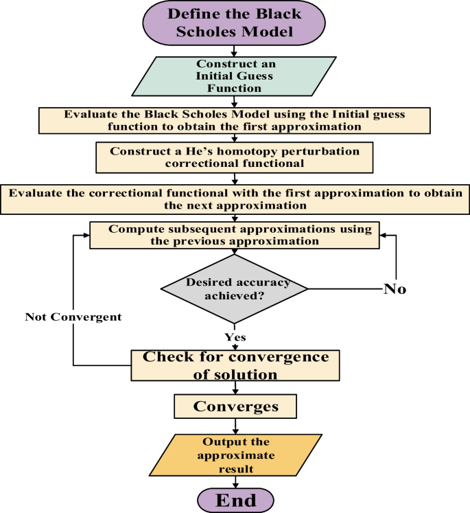

  

  Flow chat of the algorithm

2.2 Homotopy perturbation method

The following non-linear differential equation may be used to explain the basic methodology of He's homotopy perturbation method:

$$\Delta (v) - \beta (\mu ) = 0,\quad \mu \varepsilon \Omega .$$

(5)

Subject to the boundary condition:

$$B\left( {v,v_{n} } \right) = 0,\quad \mu \varepsilon \Gamma .$$

(6)

Δ represents the general differential operator, B stands for the boundary operator, β(μ) is an analytic function and Γ is the boundary operator in the domain Ω. We can separate operator Δ into two parts:

$$\Delta (v) = \ell (v) + \eta (v).$$

(7)

where $\ell$ and η denote the linear and nonlinear operator respectively. (7) into (5) yields

$$\ell (u) + \eta (u) - \beta (\mu ) = 0.$$

(8)

We can construct a homotopy for (5):

$$H(u,p) = (1 - p)\left[ {\ell (u) - \ell (v_{0} )} \right] + p\left[ {\Delta (u) - \beta (\mu )} \right] = 0,$$

(9)

simplifying (9) yields;

$$H(u,p) = \ell (u) - \ell (v_{0} ) + p\ell \left[ {u_{0} } \right] + p\left[ {\eta (u) - \beta (\mu )} \right] = 0.$$

(10)

where p is an embedded parameter which undergo deformation process of changing from 0 to 1.

At p = 0,

$$H(u,0) = \ell (u) - \ell (v_{0} ) = 0,$$

(11)

At p = 1,

$$H(u,1) = \Delta (u) - \beta (\mu ) = 0.$$

(12)

We assume a power series solution as follows:

$$u(x,t) = u_{0} (s,t) + pu_{1} (s,t) + p^{2} u_{2} (s,t) + \cdots p^{n} u_{n} (s,t),$$

(13)

Such that the approximate solution of (3) is:

$$\mathop {\lim }\limits_{p \to 1} u(s,t) = u_{0} (s,t) + u_{1} (s,t) + u_{2} (s,t) + \cdots u_{n} (s,t).$$

(14)

The convergence of this series has been proved in [23]. Substituting (13) into (1212) and equating coefficients of equal powers of p,

$$\left. \begin{gathered} p^{0} {:}u_{0} - \beta (\mu ) = 0, \hfill \\ p^{1} {:}u_{1} - H\left( {u_{0} } \right) = 0, \hfill \\ \vdots \hfill \\ p^{n} {:}u_{n} - H\left( {u_{0} ,u_{1} ,u_{2} ,u_{3} , \ldots ,u_{n - 1} } \right) = 0. \hfill \\ \end{gathered} \right\}$$

(15)

The approximate result of each iteration is obtained by solving (13).

2.3 Modified initial guess homotopy perturbation method

In this section, we illustrate the methodology and implementation of the proposed modified initial guess homotopy perturbation technique to achieve the approximate solution of a generalized fractional order black Scholes model (FOBSM) in (1) given by:

$$\frac{{\partial^{\alpha } f(s,t)}}{{\partial t^{\alpha } }} + rs\frac{\partial f(s,t)}{{\partial s}} + \frac{1}{2}\sigma^{2} s^{2} \frac{{\partial^{2} f(s,t)}}{{\partial s^{2} }} - rf(s,t) = 0,$$

(16)

Subject to initial condition:

$$f(s,0) = \max \{ s - ke^{ - rT} ,0\} = \left\{ {\begin{array}{*{20}l} {s - ke^{ - rT} ,} \hfill & {\quad s > ke^{ - rT} } \hfill \\ {0,} \hfill & {\quad {\text{otherwise}}} \hfill \\ \end{array} } \right..$$

We can construct a correctional functional using the modified initial guess homotopy perturbation method:

$$f(s,t) = f(s,0) + \sum\limits_{n = 1}^{\infty } {\lambda_{n} t^{n\alpha } } ,\quad 0 < \alpha \le 1.$$

(17)

Substituting the initial condition $f(s,0) = \max \{ s - ke^{ - rT} ,0\}$ into (17),

$$f(s,t) = \max \{ s - ke^{ - rT} ,0\} + \lambda_{1} t^{\alpha } + \lambda_{2} t^{2\alpha } + \cdots \lambda_{n} t^{n\alpha } .$$

(18)

From 188), $\lambda_{1} t^{\alpha } = f_{1} (s,t),\,\lambda_{2} t^{2\alpha } = f_{2} (s,t),$ and so on.

As an assumed solution of (1), Eq. (18) must satisfy (1) with unique values of $\lambda_{1} ,\lambda_{2} ,\lambda_{3} , \ldots \lambda_{n}$. Thus we evaluate these values, by obtaining the following derivatives:

$$\begin{aligned} f_{t} (s,t) & = \lambda_{1} \Gamma (\alpha + 1) + \lambda_{2} \frac{\Gamma (2\alpha + 1)}{{\Gamma (\alpha + 1)}}t^{\alpha } + \cdots , \\ f_{s} (s,t) & = \max \{ 1,0\} = 1, \\ f_{ss} (s,t) & = \max \{ 0,0\} = 0. \\ \end{aligned}$$

(19)

Evaluating (16) using (19),

$\lambda_{1} \Gamma (\alpha + 1) + rs - r\max \{ s - ke^{ - rT} ,0\} = 0$.

Suppose $\max \{ s - ke^{ - rT} ,0\} = (s - ke^{ - rT} )^{ + }$, then $\lambda_{1} \Gamma (\alpha + 1) + rs - r(s - ke^{ - rT} ) = 0$.

Such that $\lambda_{1} \Gamma (\alpha + 1) + kre^{ - rT} = 0 \Rightarrow \lambda_{1} = - \frac{{kre^{ - rT} }}{\Gamma (\alpha + 1)}$.

Which yields the first approximation result

$$f_{1} (s,t) = - \frac{{kre^{ - rT} }}{\Gamma (\alpha + 1)}t^{\alpha } .$$

(20)

Now we can construct a homotopy for (16) such that

$$(1 - p)\frac{{\partial^{\alpha } f(s,t)}}{{\partial t^{\alpha } }} + p\left( {\frac{{\partial^{\alpha } f(s,t)}}{{\partial t^{\alpha } }} + rs\frac{\partial f(s,t)}{{\partial s}} + \frac{1}{2}\sigma^{2} s^{2} \frac{{\partial^{2} f(s,t)}}{{\partial s^{2} }} - rf(s,t)} \right) = 0$$

(21)

Simplifying (21),

$$\frac{{\partial^{\alpha } f(s,t)}}{{\partial t^{\alpha } }} + p\left( {rs\frac{\partial f(s,t)}{{\partial s}} + \frac{1}{2}\sigma^{2} s^{2} \frac{{\partial^{2} f(s,t)}}{{\partial s^{2} }} - rf(s,t)} \right) = 0$$

(22)

We can assume a series solution for (22) such that

$$f(s,t) = f_{0} (s,t) + pf_{1} (s,t) + p^{2} f_{2} (s,t) + p^{3} f_{3} (s,t) + \cdots p^{n} f_{n} (s,t)$$

(23)

Evaluating (22) with (23) and comparing coefficients of equal powers of pⁿ, $n \ge 2$ we obtain:

$$\left. \begin{gathered} p^{2} {:}\frac{{\partial^{\alpha } f_{2} (s,t)}}{{\partial t^{\alpha } }} + rs\frac{{\partial f_{1} (s,t)}}{\partial s} + \frac{1}{2}\sigma^{2} s^{2} \frac{{\partial^{2} f_{1} (s,t)}}{{\partial s^{2} }} - rf_{1} (s,t) = 0, \hfill \\ p^{3} {:}\frac{{\partial^{\alpha } f_{3} (s,t)}}{{\partial t^{\alpha } }} + rs\frac{{\partial f_{2} (s,t)}}{\partial s} + \frac{1}{2}\sigma^{2} s^{2} \frac{{\partial^{2} f_{2} (s,t)}}{{\partial s^{2} }} - rf_{2} (s,t) = 0, \hfill \\ \vdots \hfill \\ p^{n} {:}\frac{{\partial^{\alpha } f_{n} (s,t)}}{{\partial t^{\alpha } }} + rs\frac{{\partial f_{n - 1} (s,t)}}{\partial s} + \frac{1}{2}\sigma^{2} s^{2} \frac{{\partial^{2} f_{n - 1} (s,t)}}{{\partial s^{2} }} - rf_{n - 1} (s,t) = 0, \hfill \\ \end{gathered} \right\}$$

(24)

Evaluating coefficient of p² with $f_{1} (s,t) = - \frac{{kre^{ - rT} }}{\Gamma (\alpha + 1)}t^{\alpha }$,

$$\frac{{\partial^{\alpha } f_{2} (s,t)}}{{\partial t^{\alpha } }} + \frac{{kre^{ - rT} }}{\Gamma (\alpha + 1)}t^{\alpha } = 0, \Rightarrow \frac{{\partial^{\alpha } f_{2} (s,t)}}{{\partial t^{\alpha } }} = - \frac{{kre^{ - rT} }}{\Gamma (\alpha + 1)}t^{\alpha } .$$

(25)

Applying integral operator I^α to both sides of (25), return the second approximation $f_{2} (s,t) = - \frac{{kr^{2} e^{ - rT} }}{\Gamma (2\alpha + 1)}t^{2\alpha }$. Similarly, consequent approximations can be computed for such that $f_{3} (s,t) = - \frac{{kr^{3} e^{ - rT} }}{\Gamma (3\alpha + 1)}t^{3\alpha } ,\quad f_{4} (s,t) = - \frac{{kr^{4} e^{ - rT} }}{\Gamma (4\alpha + 1)}t^{4\alpha } ,\quad f_{5} (s,t) = - \frac{{kr^{5} e^{ - rT} }}{\Gamma (5\alpha + 1)}t^{5\alpha }$, etc.

Such that the nth approximation yields $f_{n} (s,t) = - \frac{{kr^{n} e^{ - rT} }}{\Gamma (n\alpha + 1)}t^{n\alpha }$.

Thus, the approximate solution $f_{n} (s,t) = f_{0} (s,t) + f_{1} (s,t) + f_{2} (s,t) + \cdots f_{n} (s,t)$ yields

$$f_{n} (s,t) = s - ke^{ - rT} - \frac{{kre^{ - rT} }}{\Gamma (\alpha + 1)}t^{\alpha } - \frac{{kr^{2} e^{ - rT} }}{\Gamma (2\alpha + 1)}t^{2\alpha } \cdots - \frac{{kr^{n} e^{ - rT} }}{\Gamma (n\alpha + 1)}t^{n\alpha }$$

(26)

Such that

$$f_{n} (s,t) = s - ke^{ - rT} \left( {1 + \frac{{rt^{\alpha } }}{\Gamma (\alpha + 1)} + \frac{{(rt^{\alpha } )^{2} }}{\Gamma (2\alpha + 1)} + \frac{{(rt^{\alpha } )^{3} }}{\Gamma (3\alpha + 1)} \cdots + \frac{{(rt^{\alpha } )^{n} }}{\Gamma (n\alpha + 1)}} \right)$$

(27)

Which yields

$$f_{n} (s,t) = s - ke^{ - rT} \sum\limits_{q = 0}^{n} {\frac{{\left( {rt^{\alpha } } \right)^{q} }}{\Gamma (q\alpha + 1)}} .$$

(28)

At α = 1, $\sum\nolimits_{q = 0}^{\infty } {\frac{{\left( {rt^{\alpha } } \right)^{q} }}{\Gamma (q\alpha + 1)}} = e^{rt}$.

Such that (28) becomes:

$f(s,t) = s - ke^{ - r(T - t)}$ which is the exact solution of (16) as discussed in [38].

2.4 Convergence of solution

We investigated the convergence of the modified initial guess homotopy perturbation technique on the solution obtained for (16). This convergence is only based on contraction of S such that:

$$\begin{aligned} \left\| {\mu_{0} - \mu_{e} } \right\| & \le \left\| {S_{0} - S_{e} } \right\| = \left\| {s - ke^{ - rT} - (s - ke^{ - rT} \cdot ke^{rt} )} \right\| = ke^{ - rT} \left\| {e^{rt} - 1} \right\| \\ \left\| {\mu_{1} - \mu_{e} } \right\| & = \left\| {S_{0} + S_{1} - S_{e} } \right\| = ke^{ - rT} \left\| {e^{rt} - 1 - rt} \right\| \le \left\| {\mu_{0} - \mu_{e} } \right\|, \\ \left\| {\mu_{2} - \mu_{e} } \right\| & \le \left\| {S_{0} + S_{1} + S_{2} - S_{e} } \right\| = ke^{ - rT} \left\| {e^{rt} - 1 - rt - \frac{{r^{2} t^{2} }}{2}} \right\| \le \left\| {\mu_{1} - \mu_{e} } \right\|, \\ \left\| {\mu_{n} - \mu_{e} } \right\| & \le \left\| {S_{0} + S_{1} + S_{2} + \cdots S_{n} - S_{e} } \right\| = ke^{ - rT} \left\| {e^{rt} - (1 + rt + \frac{{r^{2} t^{2} }}{2} + \cdots \frac{{r^{n} t^{n} }}{n!})} \right\| \le \left\| {\mu_{n - 1} - \mu_{e} } \right\|, \\ \left\| {\mu_{n} - \mu_{e} } \right\| & \le ke^{ - rT} \left\| {e^{rt} - \left( {\sum\limits_{n = 0}^{\infty } {\frac{{r^{n} t^{n} }}{n!}} } \right)} \right\| \le \left\| {\mu_{n - 1} - \mu_{e} } \right\|, \\ \end{aligned}$$

Clearly, $\sum\nolimits_{n = 0}^{\infty } {\frac{{r^{n} t^{n} }}{n!}} = e^{rt}$, therefore $\left\| {\mu_{n} - \mu_{e} } \right\|_{\infty } \le ke^{ - rT} \left\| {ke^{rt} - ke^{rt} } \right\|_{\infty } = 0$. Thus, the contraction of $\mu_{n} (x,t)$ to μ_e as n → ∞ generated by the modified initial guess homotopy perturbation method assures that the method converges unconditionally to the exact solution.

3 Applications

This section discusses the applications of the modified initial guess homotopy perturbation method in the context of the Black–Scholes equation under various market constraints.

Problem 1

Compute the European call option of a financial asset with drift $r = \frac{5}{8}$ and volatility rate $\sigma = \frac{1}{2}$ modelled with the following Caputo fractional order Black Scholes equation:

$$\frac{{\partial^{\alpha } f(s,t)}}{{\partial t^{\alpha } }} + \frac{5}{8}s\frac{\partial f(s,t)}{{\partial s}} + \frac{1}{8}s^{2} \frac{{\partial^{2} f(s,t)}}{{\partial s^{2} }} - \frac{5}{8}f(s,t) = 0,$$

(29)

Subject to initial call option

$$f(s,0) = \max \left\{ {s^{3} ,0} \right\} = (s^{3} )^{ + } .$$

(30)

We can compute the European call option value of the model by applying the modified initial guess homotopy perturbation method. Thus a correctional formula can be constructed such that

$$f(s,t) = f(s,0) + \sum\limits_{n = 1}^{\infty } {\lambda_{n} t^{n\alpha } } ,\quad 0 < \alpha \le 1.$$

(31)

Evaluating (31) using (30) yields:

$$f(s,t) = s^{3} + \lambda_{1} t^{\alpha } + \lambda_{2} t^{2\alpha } + \cdots$$

(32)

Such that

$$\begin{aligned} f_{t} (s,t) & = \lambda_{1} \Gamma (\alpha + 1) + \lambda_{2} \frac{\Gamma (2\alpha + 1)}{{\Gamma (\alpha + 1)}}t^{\alpha } + \cdots , \\ f_{s} (s,t) & = 3s^{2} , \\ f_{ss} (s,t) & = 6s. \\ \end{aligned}$$

(33)

Evaluating (29) with (33), at t = 0;

$$\lambda_{1} \Gamma (\alpha + 1) + \frac{5}{8}s(3s^{2} ) + \frac{1}{8}s^{2} (6s) - \frac{5}{8}(s^{3} + \lambda_{1} t^{\alpha } ) = 0,$$

(34)

Which yields:

$$\lambda_{1} \Gamma (\alpha + 1) + 2s^{3} = 0, \Rightarrow \lambda_{1} = - \frac{{2s^{3} }}{\Gamma (\alpha + 1)}.$$

(35)

Such that

$$f_{1} (s,t) = \lambda_{1} t^{\alpha } = - \frac{{2s^{3} }}{\Gamma (\alpha + 1)}t^{\alpha } .$$

(36)

To obtain the subsequent approximations, we can construct a homotopy for (29):

$$(1 - p)\left[ {\frac{{\partial^{\alpha } f(s,t)}}{{\partial t^{\alpha } }}} \right] + p\left[ {\frac{{\partial^{\alpha } f(s,t)}}{{\partial t^{\alpha } }} + \frac{5}{8}s\frac{\partial f(s,t)}{{\partial s}} + \frac{1}{8}s^{2} \frac{{\partial^{2} f(s,t)}}{{\partial s^{2} }} - \frac{5}{8}f(s,t)} \right] = 0,$$

(37)

simplifying (30) yields

$$\frac{{\partial^{\alpha } f(s,t)}}{{\partial t^{\alpha } }} + p\left[ {\frac{5}{8}s\frac{\partial f(s,t)}{{\partial s}} + \frac{1}{8}s^{2} \frac{{\partial^{2} f(s,t)}}{{\partial s^{2} }} - \frac{5}{8}f(s,t)} \right] = 0,$$

(38)

Substituting (23) into (37) and comparing the coefficients of pⁿ, $n \ge 2$, we obtain:

$$p^{2} {:}\frac{{\partial^{\alpha } f_{2} (s,t)}}{{\partial t^{\alpha } }} + \frac{5}{8}s\frac{{\partial f_{1} (s,t)}}{\partial s} + \frac{1}{8}s^{2} \frac{{\partial^{2} f_{1} (s,t)}}{{\partial s^{2} }} - \frac{5}{8}f_{1} (s,t) = 0,$$

(39)

$$p^{3} {:}\frac{{\partial^{\alpha } f_{3} (s,t)}}{{\partial t^{\alpha } }} + \frac{5}{8}s\frac{{\partial f_{2} (s,t)}}{\partial s} + \frac{1}{8}s^{2} \frac{{\partial^{2} f_{2} (s,t)}}{{\partial s^{2} }} - \frac{5}{8}f_{2} (s,t) = 0,$$

(40)

$$p^{4} {:}\frac{{\partial^{\alpha } f_{4} (s,t)}}{{\partial t^{\alpha } }} + \frac{5}{8}s\frac{{\partial f_{3} (s,t)}}{\partial s} + \frac{1}{8}s^{2} \frac{{\partial^{2} f_{3} (s,t)}}{{\partial s^{2} }} - \frac{5}{8}f_{3} (s,t) = 0.$$

(41)

And so on. Evaluating (39) using (36) we obtain

$$\frac{{\partial^{\alpha } f_{2} (s,t)}}{{\partial t^{\alpha } }} - \frac{{4s^{3} t^{\alpha } }}{{\Gamma \left( {\alpha + 1} \right)}} = 0,\quad \Rightarrow \quad \frac{{\partial^{\alpha } f_{2} (s,t)}}{{\partial t^{\alpha } }} = \frac{{4s^{3} t^{\alpha } }}{{\Gamma \left( {\alpha + 1} \right)}}.$$

(42)

Applying integral operator I^α on (42) yields the second approximation obtained as:

$$f_{2} (s,t) = \frac{{4s^{3} t^{2\alpha } }}{{\Gamma \left( {2\alpha + 1} \right)}}.$$

(43)

Similar to second iteration we can evaluate (40) with (43) to obtain the third approximation:

$$\frac{{\partial^{\alpha } f_{3} (s,t)}}{{\partial t^{\alpha } }} + \frac{{8s^{3} t^{2\alpha } }}{{\Gamma \left( {2\alpha + 1} \right)}} = 0,\quad \Rightarrow \quad \frac{{\partial^{\alpha } f_{3} (s,t)}}{{\partial t^{\alpha } }} = - \frac{{8s^{3} t^{2\alpha } }}{{\Gamma \left( {2\alpha + 1} \right)}}.$$

(44)

Applying integral operator I^α on (44) yields the second approximation obtained as:

$$f_{3} (s,t) = - \frac{{8s^{3} t^{3\alpha } }}{{\Gamma \left( {3\alpha + 1} \right)}}$$

(45)

Subsequent approximations are wisely computed using Mathematica 12 software package such that,

$$f_{4} (s,t) = \frac{{16s^{3} t^{4\alpha } }}{{\Gamma \left( {4\alpha + 1} \right)}},\quad f_{5} (s,t) = - \frac{{32s^{3} t^{5\alpha } }}{{\Gamma \left( {5\alpha + 1} \right)}}, \cdots$$

(46)

Such that the approximate solution

$$f(s,t) = \sum\limits_{n = 0}^{\infty } {f_{n} (s,t)} = s^{3} - \frac{{2s^{3} t^{\alpha } }}{{\Gamma \left( {\alpha + 1} \right)}} + \frac{{4s^{3} t^{2\alpha } }}{{\Gamma \left( {2\alpha + 1} \right)}} - \frac{{8s^{3} t^{3\alpha } }}{{\Gamma \left( {3\alpha + 1} \right)}} + \frac{{16s^{3} t^{4\alpha } }}{{\Gamma \left( {4\alpha + 1} \right)}} + \cdots ( - 1)^{n} \frac{{s^{3} \left( {2t^{\alpha } } \right)^{n} }}{{\Gamma \left( {n\alpha + 1} \right)}}$$

(47)

Such that

$$f(s,t) = \sum\limits_{n = 0}^{\infty } {f_{n} (s,t)} = s^{3} \left( {\sum\limits_{n = 0}^{\infty } {\frac{{( - 1)^{n} \left( {2t^{\alpha } } \right)^{n} }}{{\Gamma \left( {n\alpha + 1} \right)}}} } \right).$$

(48)

The integer solution can be obtained when α = 1:

$$f(s,t) = \sum\limits_{n = 0}^{\infty } {f_{n} (s,t)} = s^{3} \sum\limits_{n = 0}^{\infty } {\frac{{( - 1)^{n} \left( {2t} \right)^{n} }}{{\Gamma \left( {n + 1} \right)}}} .$$

(49)

Now, modified initial guess agrees that:

$$\mathop {\lim }\limits_{n \to \infty } f_{n} (s,t) = f(s,t),$$

Thus, at an integer order the exact payoff value for the European call option in (29) is:

$$f(s,t) = s^{3} e^{ - 2t} .$$

(50)

Problem 2

Consider a financial asset with a free interest and stock market volatility rate equilibrium specified by m = 5. Modeled using the Caputo fractional order black Scholes model,

$$\frac{{\partial^{\alpha } v(s,t)}}{{\partial t^{\alpha } }} - \frac{{\partial^{2} v(s,t)}}{{\partial s^{2} }} - 4\frac{\partial v(s,t)}{{\partial s}} + 5v(s,t) = 0$$

(51)

Subject to initial condition

$$v(s,0) = \max \{ e^{s} - 1,0\} = (e^{s} - 1)^{ + }$$

(52)

By modified initial guess, we construct the correctional functional:

$$v(s,t) = v(s,0) + \lambda_{1} t^{\alpha } + \lambda_{2} t^{2\alpha } + \lambda_{3} t^{3\alpha } + \cdots ,\quad 0 < \alpha \le 1.$$

(53)

Substituting (52) into (53), we obtain

$$v(s,t) = (e^{s} - 1) + \lambda_{1} t^{\alpha } + \lambda_{2} t^{2\alpha } + \lambda_{3} t^{3\alpha } + \cdots ,\quad 0 < \alpha \le 1.$$

(54)

Equation (54) is applied in evaluating (51) such that we obtain:

$$\lambda_{1} \Gamma \left( {\alpha + 1} \right) - e^{s} - 4e^{s} + 5(e^{s} - 1 + \lambda_{1} t^{\alpha } + \lambda_{2} t^{2\alpha } + \cdots ) = 0$$

(55)

Evaluating (55) at t = 0, and simplifying, we obtain:

$$\lambda_{1} \Gamma \left( {\alpha + 1} \right) - 5 = 0\quad \Rightarrow \quad \lambda_{1} = \frac{5}{{\Gamma \left( {\alpha + 1} \right)}}.$$

(56)

Such that

$$u_{1} (s,t) = \lambda_{1} t^{\alpha } = \frac{{5t^{\alpha } }}{{\Gamma \left( {\alpha + 1} \right)}}$$

(57)

Constructing a homotopy for (51) to obtain subsequent approximations,

$$(1 - p)\left[ {\frac{{\partial^{\alpha } v(s,t)}}{{\partial t^{\alpha } }}} \right] + p\left[ {\frac{{\partial^{\alpha } v(s,t)}}{{\partial t^{\alpha } }} - \frac{{\partial^{2} v(s,t)}}{{\partial s^{2} }} - 4\frac{\partial v(s,t)}{{\partial s}} + 5v(s,t)} \right] = 0$$

(58)

Evaluating (58) with (23) and comparing the coefficients of pⁿ, $n \ge 2$, we obtain:

$$p^{2} {:}\frac{{\partial^{\alpha } v_{2} (s,t)}}{{\partial t^{\alpha } }} - \frac{{\partial^{2} v_{1} (s,t)}}{{\partial s^{2} }} - 4\frac{{\partial v_{1} (s,t)}}{\partial s} + 5v_{1} (s,t) = 0,$$

(59)

$$p^{3} {:}\frac{{\partial^{\alpha } v_{3} (s,t)}}{{\partial t^{\alpha } }} - \frac{{\partial^{2} v_{2} (s,t)}}{{\partial s^{2} }} - 4\frac{{\partial v_{2} (s,t)}}{\partial s} + 5v_{2} (s,t) = 0,$$

(60)

$$p^{4} {:}\frac{{\partial^{\alpha } v_{4} (s,t)}}{{\partial t^{\alpha } }} - \frac{{\partial^{2} v_{3} (s,t)}}{{\partial s^{2} }} - 4\frac{{\partial v_{3} (s,t)}}{\partial s} + 5v_{3} (s,t) = 0.$$

(61)

And so on. The second approximation can be obtained by evaluating (59) with (57):

$$\frac{{\partial^{\alpha } v_{2} (s,t)}}{{\partial t^{\alpha } }} + \frac{{25t^{\alpha } }}{{\Gamma \left( {\alpha + 1} \right)}} = 0,\quad \Rightarrow \quad \frac{{\partial^{\alpha } v_{2} (s,t)}}{{\partial t^{\alpha } }} = - \frac{{25t^{\alpha } }}{{\Gamma \left( {\alpha + 1} \right)}}$$

(62)

Applying the integral operator I^α on both sides of (62) yields the required approximate value:

$$v_{2} (s,t) = - \frac{{25t^{2\alpha } }}{{\Gamma \left( {2\alpha + 1} \right)}}$$

(63)

The third approximation can similarly be computed by evaluating (60) using (63) such that,

$$\frac{{\partial^{\alpha } v_{3} (s,t)}}{{\partial t^{\alpha } }} - \frac{{125t^{2\alpha } }}{{\Gamma \left( {2\alpha + 1} \right)}} = 0,\quad \Rightarrow \quad \frac{{\partial^{\alpha } v_{3} (s,t)}}{{\partial t^{\alpha } }} = \frac{{125t^{2\alpha } }}{{\Gamma \left( {2\alpha + 1} \right)}}$$

(64)

Operator I^α can be applied on both sides of (64) to obtain the third approximation such that

$$v_{3} (s,t) = \frac{{125t^{3\alpha } }}{{\Gamma \left( {3\alpha + 1} \right)}}$$

(65)

Repeating the iterative procedure, the following results are achieved as successive approximations:

$$v_{4} (s,t) = - \frac{{625t^{4\alpha } }}{{\Gamma \left( {4\alpha + 1} \right)}},v_{5} (s,t) = + \frac{{3125t^{5\alpha } }}{{\Gamma \left( {5\alpha + 1} \right)}}, \cdots$$

Such that the approximate solution $v(s,t) = v_{0} (s,t) + v_{1} (s,t) + v_{2} (s,t) + \cdots v_{n} (s,t)$ yields

$$v(s,t) = \sum\limits_{n = 0}^{\infty } {v_{n} (s,t) = } e^{s} - 1 + \frac{{5t^{\alpha } }}{{\Gamma \left( {\alpha + 1} \right)}} - \frac{{25t^{2\alpha } }}{{\Gamma \left( {2\alpha + 1} \right)}} + \frac{{125t^{3\alpha } }}{{\Gamma \left( {3\alpha + 1} \right)}} - \frac{{625t^{4\alpha } }}{{\Gamma \left( {4\alpha + 1} \right)}} + \frac{{3125t^{5\alpha } }}{{\Gamma \left( {5\alpha + 1} \right)}} + \cdots$$

(66)

Taking the sum, we obtain

$$v(s,t) = \sum\limits_{n = 0}^{\infty } {v_{n} (s,t) = } e^{s} - \sum\limits_{n = 0}^{\infty } {\frac{{\left( { - 1} \right)^{n} \left( {5t^{\alpha } } \right)^{n} }}{{\Gamma \left( {n\alpha + 1} \right)}}}$$

(67)

The integer solution can be obtained at α = 1:

$$v(s,t) = \sum\limits_{n = 0}^{\infty } {v_{n} (s,t) = } e^{s} - \sum\limits_{n = 0}^{\infty } {\frac{{\left( { - 1} \right)^{n} \left( {5t} \right)^{n} }}{{\Gamma \left( {n + 1} \right)}}}$$

(68)

The modified initial guess approach agrees that:

$$\mathop {\lim }\limits_{n \to \infty } v_{n} (s,t) = v(s,t)$$

Thus at an integer order, the exact solution of the Fractional order Black Scholes model in (51) is:

$$v(s,t) = e^{s} - e^{ - 5t} .$$

(69)

This indeed is the solution of (4) presented in [31] at a value of m = 5 provided that

$$v_{\max } = (e^{s} - 1)^{ + } e^{ - kt} + (e^{s} )^{ + } (1 - e^{ - kt} ),$$

in their obtained result given as:

$$v(s,t) = \max \{ e^{s} - 1,0\} e^{ - mt} + \max \{ e^{s} ,0\} (1 - e^{ - mt} ).$$

Problem 3

Compute the European put option of an asset with a drift value r = 0.24 and a dynamic volatility rate $\sigma = 0.6(\cos \,s)$ modelled with the following Black Scholes model:

$$\frac{{\partial^{\alpha } u(s,t)}}{{\partial t^{\alpha } }} + 0.18(\cos^{2} s)s^{2} \frac{{\partial^{2} u(s,t)}}{{\partial s^{2} }} + 0.24s\frac{\partial v(s,t)}{{\partial s}} - 0.24u(s,t) = 0$$

(70)

Subject to initial condition:

$$u(s,0) = \max \{ s - 16e^{ - 0.24} ,0\} = (s - 16e^{ - 0.24} )^{ + }$$

(71)

A correctional functional is constructed for (70):

$$u(s,t) = u(s,0) + \lambda_{1} t^{\alpha } + \lambda_{2} t^{2\alpha } + \lambda_{3} t^{3\alpha } + \cdots \quad 0 < \alpha \le 1.$$

(72)

Substituting (71) into (72) yields

$$u(s,t) = s - 16e^{ - 0.24} + \lambda_{1} t^{\alpha } + \lambda_{2} t^{2\alpha } + \lambda_{3} t^{3\alpha } + \cdots .$$

(73)

Evaluating (70) using (71) yields:

$$\lambda_{1} \Gamma \left( {\alpha + 1} \right) + 0.24s - 0.24(s - 16e^{ - 0.24} + \lambda_{1} t^{\alpha } + \lambda_{2} t^{2\alpha } + \lambda_{3} t^{3\alpha } + \cdots .) = 0;$$

Thus at t = 0, (772 becomes:

$$\lambda_{1} \Gamma \left( {\alpha + 1} \right) + 0.24 \times 16e^{ - 0.24} = 0$$

(74)

Solving for λ₁ yields

$$\lambda_{1} = - \frac{{0.24 \times 16e^{ - 0.24} }}{{\Gamma \left( {\alpha + 1} \right)}}.$$

(75)

Such that the first approximation yields;

$$u_{1} (s,t) = \lambda_{1} t^{\alpha } = - \frac{{0.24 \times 16e^{ - 0.24} }}{{\Gamma \left( {\alpha + 1} \right)}}t^{\alpha }$$

(76)

We can construct a homotopy for (70) to obtain proceeding approximations such that:

$$(1 - p)\left[ {\frac{{\partial^{\alpha } u(s,t)}}{{\partial t^{\alpha } }}} \right] + p\left[ {\frac{{\partial^{\alpha } u(s,t)}}{{\partial t^{\alpha } }} + 0.18(\cos s)^{2} s^{2} \frac{{\partial^{2} u(s,t)}}{{\partial s^{2} }} + 0.24s\frac{\partial v(s,t)}{{\partial s}} - 0.24u(s,t)} \right] = 0$$

(77)

Substituting (23) into (77) and comparing the coefficients of pⁿ, $n \ge 2$, we obtain:

$$p^{2} {:}\frac{{\partial^{\alpha } u_{2} (s,t)}}{{\partial t^{\alpha } }} + 0.18(\cos s)^{2} s^{2} \frac{{\partial^{2} u_{1} (s,t)}}{{\partial s^{2} }} + 0.24s\frac{{\partial u_{1} (s,t)}}{\partial s} - 0.24u_{1} (s,t) = 0$$

(78)

$$p^{3} {:}\frac{{\partial^{\alpha } u_{3} (s,t)}}{{\partial t^{\alpha } }} + 0.18(\cos s)^{2} s^{2} \frac{{\partial^{2} u_{2} (s,t)}}{{\partial s^{2} }} + 0.24s\frac{{\partial u_{2} (s,t)}}{\partial s} - 0.24u_{2} (s,t) = 0$$

(79)

$$p^{4} {:}\frac{{\partial^{\alpha } u_{4} (s,t)}}{{\partial t^{\alpha } }} + 0.18(\cos s)^{2} s^{2} \frac{{\partial^{2} u_{3} (s,t)}}{{\partial s^{2} }} + 0.24s\frac{{\partial u_{3} (s,t)}}{\partial s} - 0.24u_{3} (s,t) = 0$$

(80)

And so on. The second approximation result is obtained by evaluating (78) by (76):

$$\frac{{\partial^{\alpha } u_{2} (s,t)}}{{\partial t^{\alpha } }} + 0.24 \times \frac{{0.24 \times 16e^{ - 0.24} }}{{\Gamma \left( {\alpha + 1} \right)}}t^{\alpha } = 0\quad \Rightarrow \quad \frac{{\partial^{\alpha } u_{2} (s,t)}}{{\partial t^{\alpha } }} = - \frac{{(0.24)^{2} \times 16e^{ - 0.24} }}{{\Gamma \left( {\alpha + 1} \right)}}t^{\alpha }$$

(81)

Applying operator I^α on both sides of (81), we obtain

$$u_{2} (s,t) = - \frac{{(0.24)^{2} \times 16e^{ - 0.24} }}{{\Gamma \left( {2\alpha + 1} \right)}}t^{2\alpha }$$

(82)

Repeating the same process for (79), to obtain u₃(x, t),

$$\frac{{\partial^{\alpha } u_{3} (s,t)}}{{\partial t^{\alpha } }} + 0.24 \times \frac{{(0.24)^{2} \times 16e^{ - 0.24} }}{{\Gamma \left( {2\alpha + 1} \right)}}t^{2\alpha } = 0\quad \Rightarrow \quad \frac{{\partial^{\alpha } u_{3} (s,t)}}{{\partial t^{\alpha } }} = - \frac{{(0.24)^{3} \times 16e^{ - 0.24} }}{{\Gamma \left( {2\alpha + 1} \right)}}t^{2\alpha }$$

(83)

Also applying I^α on both sides of (83) yields the third approximation obtained as

$$u_{3} (s,t) = - \frac{{(0.24)^{3} \times 16e^{ - 0.24} }}{{\Gamma \left( {3\alpha + 1} \right)}}t^{3\alpha }$$

(84)

Subsequent approximations are computed such that

$$\left. {\begin{array}{*{20}l} {u_{4} (s,t) = - \frac{{(0.24)^{4} \times 16e^{ - 0.24} }}{{\Gamma \left( {4\alpha + 1} \right)}}t^{4\alpha } ,} \hfill \\ {u_{5} (s,t) = - \frac{{(0.24)^{5} \times 16e^{ - 0.24} }}{{\Gamma \left( {5\alpha + 1} \right)}}t^{5\alpha } ,} \hfill \\ {u_{6} (s,t) = - \frac{{(0.24)^{6} \times 16e^{ - 0.24} }}{{\Gamma \left( {6\alpha + 1} \right)}}t^{6\alpha } \cdots } \hfill \\ \end{array} } \right\}$$

(85)

Such that the approximate solution $u(s,t) = u_{0} (s,t) + u_{1} (s,t) + u_{2} (s,t) + \cdots u_{n} (s,t)$ yields

$$u(s,t) = \sum\limits_{n = 0}^{\infty } {u_{n} (s,t) = } \left. \begin{gathered} s - 16e^{ - 0.24} - \frac{{0.24 \times 16e^{ - 0.24} }}{{\Gamma \left( {\alpha + 1} \right)}}t^{\alpha } - \frac{{(0.24)^{2} \times 16e^{ - 0.24} }}{{\Gamma \left( {2\alpha + 1} \right)}}t^{2\alpha } - \frac{{(0.24)^{3} \times 16e^{ - 0.24} }}{{\Gamma \left( {3\alpha + 1} \right)}}t^{3\alpha } \hfill \\ - \frac{{(0.24)^{4} \times 16e^{ - 0.24} }}{{\Gamma \left( {4\alpha + 1} \right)}}t^{4\alpha } - \frac{{(0.24)^{5} \times 16e^{ - 0.24} }}{{\Gamma \left( {5\alpha + 1} \right)}}t^{5\alpha } - \frac{{(0.24)^{6} \times 16e^{ - 0.24} }}{{\Gamma \left( {6\alpha + 1} \right)}}t^{6\alpha } + \cdots \hfill \\ \end{gathered} \right\}$$

(86)

The sum can be taken such that the payoff function of the put option is:

$$u_{n} (s,t) = s - 16e^{ - 0.24} \sum\limits_{n = 0}^{\infty } {\frac{{(0.24t^{\alpha } )^{n} }}{{\Gamma \left( {n\alpha + 1} \right)}}}$$

The integer solution can be obtained at α = 1:

$$u_{n} (s,t) = \sum\limits_{n = 0}^{\infty } {u_{n} (s,t) = } s - 16e^{ - 0.24} \sum\limits_{n = 0}^{\infty } {\frac{{(0.24t)^{n} }}{{\Gamma \left( {n + 1} \right)}}}$$

(87)

The modified initial guess approach agrees that:

$$\mathop {\lim }\limits_{n \to \infty } u_{n} (s,t) = u(s,t)$$

Thus, the exact

$$u(s,t) = s - 16e^{ - 0.24(1 - t)} .$$

4 Results

The numerical table of results obtained by solving the fractional order Black Scholes differential equation using the proposed approach is presented in this section. In addition, to develop an insight of the price evolution of options, we run numerical simulations of the solved examples using the computational software program Maple 18, and the results are graphically presented.

Table 1 shows the numerical results of the MIGHPM, exact solution and the absolute errors. It could be observed that the results produced by the MIGHPM are in good agreement with the exact solution. Although slight deviations of the approximate results from the exact solution were observed as the value of t increases from 0 to 1. For example, the absolute error observed when t = 0, are zero 0 but at t = 0.2 the absolute errors are in order of × 10⁻¹² to × 10⁻¹⁰; and at t = 1 the absolute error increases to an order which exist in the range of × 10⁻⁴ to × 10⁻³.

Table 1 Numerical Results of problem one at an exact value α = 1

Table 2 shows that the absolute error drastically increases as t increases. We observed that, the absolute error is zero when t = 0 and the error ranges from an order of × 10⁻¹³ to × 10⁻² as t progresses from 0 to 1.

Table 2 Numerical Results of problem Two at an exact value α = 1

Table 3 shows the effectiveness of the MIGHPM in solving fractional order Black Scholes Model. It could be observed that the maximum absolute error recorded exist in the range of × 10⁻¹⁸ and the absolute error is zero at t = 0 and t = 1.

Table 3 Numerical Results of problem Three at an exact value α = 1

5 Discussion

The primary objective of this research is to ascertain the impact of Caputo fractional order derivatives on the price dynamics of financial assets. To achieve this, we examined the behavior of payoff functions concerning fluctuations in stock prices within the range of 0 < α < 1. The results of our investigation are presented as payoff curves.

Figure 2 displays the maturity graphs of option payoffs for problem 1 at various Caputo fractional order levels. Notably, for the assets under consideration, we observed a significant decline in option payout values as the maturity date approached. Specifically, in Fig. 2A, when α = 0.25, the payoff value was 40, but this sharply dropped to 3 as α increased to 0.5, and subsequently decreased further to 1 when α = 0.75, reaching parity with the exact option price. It is worth highlighting that the call value of the financial asset was found to be at its lowest when α took an integer value, signifying a market phenomenon when all constraints were fully enforced. Figure 2E provides a graphical comparison of the call option payoffs, clearly illustrating the diminishing trend as α increases. Figure 2F, on the other hand, compares the accuracy of our proposed method with the exact solution. Our findings indicate that the proposed method effectively addressed the problem, yielding an approximation result that unconditionally converges to the exact solution. Notably, our outcomes align with the results presented by Esekon et al. [38] in a prior study, where an analytical method was employed to compute the results of the classical Black–Scholes model, underscoring the efficacy of MIGHPM. Additionally, Fig. 3 depict the dynamic behavior of price evolution for the financial asset modeled in problem 2 using the Black–Scholes equation. In Fig. 3A, the payoff value is 6000 when α = 0.25, but this reduces to 2500 as α increases to 0.5 in Fig. 3B, further declining to 300 as α reaches 0.75 in Fig. 3C, ultimately converging to 4 in the exact solution presented in Fig. 3D. These results underscore the importance of exercising caution when dealing with option prices as they approach their expiration dates. Figure 3E offers a comparative plot of these factors, while Fig. 3F reaffirms the effectiveness of our method in solving the fractional order Black–Scholes equation. These findings also align with those of Edeki et al. [33], which introduced a Black–Scholes equation with constant elasticity variance for stock option evaluation. Moving on to problem 3, we present the put option's payout values in Fig. 4. Interestingly, we observed that the asset's put option similarly relies on the derivative of Caputo's fractional order. Figure 4A–C depict a substantial reduction in the asset's payoff value as α approaches the exact solution, in line with the results from [22] that employed the Lagrange multiplier method. Notably, Fig. 4C, D record negative put option payoffs as the option nears its expiration time, indicating investor losses, and the necessity to pay the absolute value of the payoff. Finally, we present graphs comparing the precise and approximate solutions of our proposed method with those generated by the built-in RK4 of Maple 18 in Fig. 4F. Despite some variations in the intervals at which RK4 Maple 18 provides option call values, we found that all three outcomes generally agree. This consistency arises from the dependence of the dynamic volatility rate on the asset price, as described in the problem statement.

Fig. 2

Graphical results of Example 1

Fig. 3

Graphical results of Example 2

Fig. 4

Graphical results of Example 3

6 Conclusions

We present a method for solving the fractional order Black Scholes model that is simple, effective, and computationally efficient. As observed in its application in [24] for obtaining the analytical solitons of fractional order Korteweg-De-Vries equation, the approach similarly demonstrates its effectiveness in solving the class of problems solved in this study as it generates an unconditionally convergent series of arbitrary order which agree with the exact solutions of the problems solved at an integer order. The investigation of the influence of the Caputo fractional order derivatives in gaining insight into the market dynamics of options price evolution is also detailed in the paper. This same Caputo derivative was investigated in a similar but distinct study presented in [21] to study dividend payments on paying financial assets modeled with the Black Scholes equation utilizing an implicit finite difference approach for solving the resultant BS-PDE. Theoretical analysis of their research essentially confirms that Caputo fractional order derivatives are the most effective way to simulate option premiums, which deviate significantly from what is predicted by classical differential operator theory. Another significant aspect to keep in mind is that the conventional BS models are known to generate option premium curves with identical curves, which may not accurately reflect the market dynamics. However, the option premium curves produced by the model developed using Caputo fractional derivatives are extremely sensitive to changes in related market characteristics, such as volatility and rates, etc.

7 Recommendation

Future research could be carried out to investigate the influence of other non-local fractional order operator such as Caputo–Fabrizo [14] and Atangana–Baleanu [15] derivatives on Black Scholes model derived from real market situations using the method applied in this study to better comprehend and forecast the dynamics of option price evolution.

References

Black F, Scholes M (1973) The pricing of options and corporate liabilities. J Polit Econ 81(3):637–654. https://doi.org/10.1086/260062.S2CID154552078
Hull JC (1997) Options, futures, and other derivatives. Prentice Hall
Merton RC (1973) Theory of rational option pricing. Bell J Econ Manag Sci 4(1):141–183. https://doi.org/10.2307/3003143
Muriel N, Fernández-Anaya G (2022) A modified Black–Scholes–Merton model for option pricing. Mathematics 10:1492. https://doi.org/10.3390/math10091492
Nurul Anwar M, Sazzad Andallah L (2018) A study on numerical solution of Black–Scholes model. J Math Finance 8:372–381. https://doi.org/10.4236/jmf.2018.82024
De Staelen RH, Hendy AS (2017) Numerically pricing double barrier options in a time-fractional Black–Scholes model. Comput Math Appl 74(6):1166–1175. https://doi.org/10.1016/j.camwa.2017.06.005
Ouafoudi M, Gao F (2018) Exact solution of fractional Black–Scholes European option pricing equations. Appl Math 9:86–100
Olayiwola MO, Alaje AI, Olarewaju AY, Adedokun KA (2023) A Caputo fractional order epidemic model for evaluating the effectiveness of high-risk quarantine and vaccination strategies on the spread of COVID-19. Healthc Anal 3:100179
Olayiwola MO, Adedokun KA (2023) A novel tuberculosis model incorporating a Caputo fractional derivative and treatment effect via the homotopy perturbation method. Bull Natl Res Centre 47(1):121
Alaje AI, Olayiwola MO (2023) A fractional-order mathematical model for examining the spatiotemporal spread of COVID-19 in the presence of vaccine distribution. Healthc Anal 4:100230
Kolawole MK, Olayiwola MO, Alaje AI, Adekunle HO, Odeyemi KA (2023) Conceptual analysis of the combined effects of vaccination, therapeutic actions, and human subjection to physical constraint in reducing the prevalence of COVID-19 using the homotopy perturbation method. Beni-Suef Univ J Basic Appl Sci 12(1):10
Liouville J (1832) Mémoire sur le calcul des différentielles à indices quelconques. Journal de l’École Polytechnique 13:71–162
Caputo M (1969) Elasticita e dissipazione. Zanichelli, Bologna
Caputo M, Fabrizio M (2016) A new definition of fractional derivative without singular kernel. Prog Fract Differ Appl 1(2):73–85
Atangana A, Baleanu D (2016) New fractional derivatives with non-local and nonsingular kernel theory and application to heat transfer model. Therm Sci 20:763–769
Veeresha P, Yavuz M, Baishya C (2021) A computational approach for shallow water forced Korteweg–De Vries equation on critical flow over a hole with three fractional operators. Int J Optim Control Theor Appl 11:52–67. https://doi.org/10.11121/ijocta.2021.1177
Edeki SO, Ugbebor OO, Owoloko EA (2017) Analytical solutions of the time-fractional order Black–Scholes model for stock option valuation on no dividend yield basis. IAENG Int J Appl Math 47(4):1–12
Yunus AO, Olayiwola MO, Adedokun KA, Adedeji JA, Alaje AI (2022) Mathematical analysis of fractional-order Caputo’s derivative of coronavirus disease model via Laplace Adomian decomposition method. Beni-Suef Univ J Basic Appl Sci 11:144. https://doi.org/10.1186/s43088-022-00326-9
Bahaa G (2017) Fractional optimal control problem for a differential system with a delay argument. Adv Diff Equ 6:66. https://doi.org/10.1186/s13662-017-1121-6
Bahaa GM (2018) Fractional optimal control problem for variational inequalities with control constraints. IMA J Math Control Inf 35(1):107–122. https://doi.org/10.1093/imamci/dnw040
Nuugulu SM, Gideon F and Patidar KC (2021) A robust numerical solution to a time-fractional Black–Scholes equation. Adv Differ Equ 123. https://doi.org/10.1186/s13662-021-03259-2.
Ghandehari MAM, Rajbar M (2014) European option pricing of fractional Black–Scholes model with new Lagrange multipliers. Comput Methods Differ Equ 2(1):1–10
He JH (1999) Homotopy perturbation technique. Comput Methods Appl Mech Eng 178:257–262
Alaje AI, Olayiwola MO, Adedokun KA, Adedeji JA, Oladapo A (2022) Modifed homotopy perturbation method and its application to analytical solitons of fractional-order Korteweg–de Vries equation. Beni-Suef Univ J Basic Appl Sci 11(39):66. https://doi.org/10.1186/s43088-022-00317-w
Sumar S, Kumar D, Singh J (2014) Numerical computation of fractional Black–Scholes equation arising in financial market. Egypt J Basic Appl Sci 1:177–183
Alaje AI, Olayiwola MO, Ogunniran MO, Adedeji JA, Adedokun KA (2021) Approximate analytical methods for the solution of fractional order integro-differential equations. Niger J Math Appl 31(2021):175–190
Yavuz M, Özdemir N (2018) A different approach to the European option pricing model with new fractional operator. Math Model Nat Phenom. https://doi.org/10.1051/mmnp/2018009
Olayiwola MO, Gbolagade AW, Adesanya AO (2010) Solving variable coefficient fourth-order parabolic equation by modified initial guess variational iteration method. J Niger Assoc Math Phys 16:205–210
Olayiwola MO, Gbolagade AW, Adesanya AO (2010) An efficient algorithm for solving the telegraph equation. J Niger Assoc Math Phys 16:199–204
Olayiwola MO, Gbolagade AW, Akinpelu FO (2011) An efficient algorithm for solving the nonlinear PDE. Int J Sci Eng Res 2:1–10
Edeki SO, Jena RM, Chakraverty S, Baleanu D (2020) Coupled transform method for time-space fractional Black–Scholes option pricing model. Alex Eng J 59(5):3239–3246. https://doi.org/10.1016/j.aej.2020.08.031
Edeki SO, Owoloko EA, Ugebor O (2016) The modified Black–Scholes model via constant elasticity of variance for stock options valuation. AIP Conf Proc. https://doi.org/10.1063/1.4940289020041
Owoyemi AE, Sumiati I, Sukono ER (2020) Laplace decomposition method for solving fractional Black Scholes European option pricing. Int J Quant Res Model 1(4):194–207
Kumar S, Yildirim A, Khan Y, Jafari H, Sayevand L, Wei I (2012) analytical solution of fractional Black–Scholes European option pricing equation by using Laplace transform. J Fract Calc Appl 2(8):1–9
Fall AN, Ndiaye SN, Sene N (2019) Black–Scholes option pricing equations described by the Caputo generalized fractional derivative. Chaos Solitons Fract 125:108–118. https://doi.org/10.1016/j.chaos.2019.05.024
Bahaa GM (2017) Fractional optimal control problem for variable-order differential systems. Fract Calc Appl Anal 20:1447–1470. https://doi.org/10.1515/fca-2017-0076
Biazar J, Ghazvini H (2009) Convergence of the homotopy perturbation method for partial differential equations. Nonlinear Anal Real World Appl 10:2633–2640
Esekon JE (2013) Analytic solution of nonlinear Black Scholes equation. Int J Pure Appl Math 82(4):547–555. https://doi.org/10.12732/ijpam.v82i4.4
Acknowledgements
The efforts of all academic colleagues in the Department of Mathematical sciences of Osun State university, Osogbo is acknowledged.
Funding
No funding has been received.
Author information
Authors and Affiliations
Contributions
A.I.—method development; M.O.—problems formulation; K.A.—Computation; J.A.—results simulation; Y.O.—Error Analysis; A.O.—Typesetting and proof reading. All authors read and approved the final manuscript.
Corresponding author
Ethics declarations
Ethics approval and consent to participate
Not applicable.
Consent for publication
Competing interests
The authors declare there are no competing interests.
Additional information
Publisher's Note
Springer Nature remains neutral with regard to jurisdictional claims in published maps and institutional affiliations.
Rights and permissions
Open Access This article is licensed under a Creative Commons Attribution 4.0 International License, which permits use, sharing, adaptation, distribution and reproduction in any medium or format, as long as you give appropriate credit to the original author(s) and the source, provide a link to the Creative Commons licence, and indicate if changes were made. The images or other third party material in this article are included in the article's Creative Commons licence, unless indicated otherwise in a credit line to the material. If material is not included in the article's Creative Commons licence and your intended use is not permitted by statutory regulation or exceeds the permitted use, you will need to obtain permission directly from the copyright holder. To view a copy of this licence, visit http://creativecommons.org/licenses/by/4.0/.
About this article
Cite this article
Alaje, A.I., Olayiwola, M.O., Adedokun, K.A. et al. The modified homotopy perturbation method and its application to the dynamics of price evolution in Caputo-fractional order Black Scholes model. Beni-Suef Univ J Basic Appl Sci 12, 93 (2023). https://doi.org/10.1186/s43088-023-00433-1
Received:
Accepted:
Published:
DOI: https://doi.org/10.1186/s43088-023-00433-1